In this AI workshop, you are going to build a model to predict the bike demand for a specific hour of a day for the city of Washington. The data is available as sample data in the Azure ML Studio (classic) and is based on the data that has been collected in 2011 and 2012 in Washington.

The dataset contains whether information and the number of bikes that have been rented. More information can be found on the UCI Machine Learning repository site: https://archive.ics.uci.edu/ml/datasets/bike+sharing+dataset

We highly recommend you visit that site and investigate what kind of data you have available.

Note: this workshop is to get in touch with machine learning. We won’t pretend to build an excellent model in 1 hour. In the real world you would have to do a lot more, but this workshop does give you an idea about the steps, with the free option of the Microsoft Azure Machine Learning Studio (classic).

Steps to build the model

You are going to build a prediction model to predict the bike demand for a specific hour of the day.

You will first open the online environment where you will build your model. Then you will select the dataset and inspect the data. Next, you will select the required columns and transform them if needed. Then you will split the dataset into 2 parts: 1 part to train the model with, and 1 to test the model with. You will train the model and use this model to score the test dataset. Finally, you will evaluate the model.

Please read the complete tutorial so you have an overview of what you will be doing.

The pictures are not very sharp, but you can download the pdf version of this workshop here to get a better view.

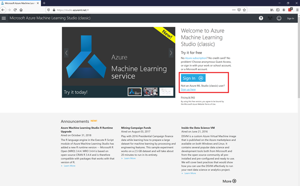
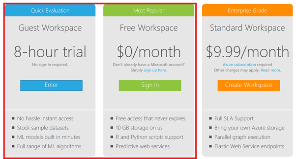
Step 1: Get access to the environment

Go to https://studio.azureml.net/ and select Sign up here for Azure ML Studio. For this workshop, you can select the 8-hour trial.

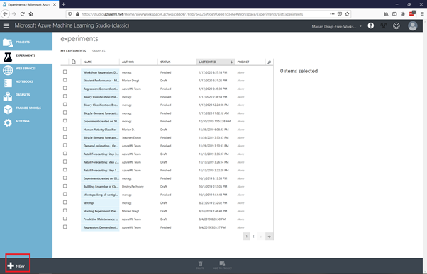
Step 2: Create a new blank Experiment and give it a name

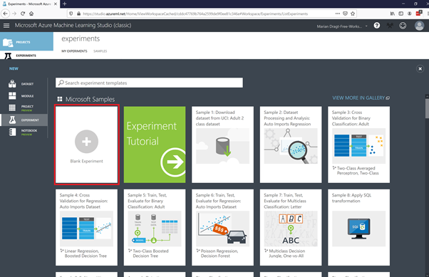
To build your model, you first have to create a new experiment. An experiment is like an instance of your model. It will open a canvas where you can drag your modules on to build your model and run it. Create a new blank experiment by clicking on the + NEW button at the left bottom corner of the screen. Now select the Blank Experiment.

This will open a canvas where you can build your model. First give your model a name. You can select the title and change it.

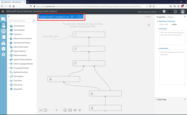
At the left, you have a menu with all kind of modules to build your model with.

Step 3: Get and visualize the data

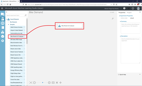
We start with the data. You can open the Saved Datasets item, select the Bike Rental UCI dataset, and drag it on the canvas.

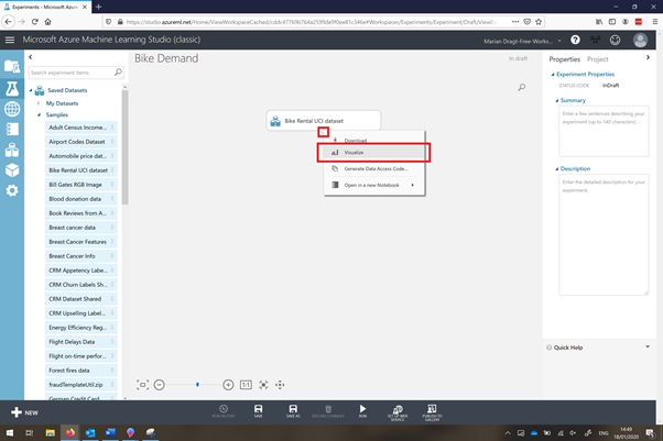
To get a quick overview of the data, you can right-click the output port and select the option Visualize. This will show you some quick insights regarding the data, like the amount of observations and variables, and the shape of the data.

As you could read at the UCI Machine Learning repository page, this dataset contains the count of usual users (column ‘casual’), registered users (column ‘registered’), and the total amount of rented bikes (column ‘cnt’). For this model we are only going to use the latter. Furthermore, we don’t need the instant variable.

Step 4: Select the required data

To select the required columns, you can use the Select Columns in Dataset module, which you can find under Manipulation in the left menu. You can connect the output port of the Bike Rental UCI dataset module with the input port of the Select Columns in Dataset module (use your mouse to draw a line between the modules). You will see a red exclamation mark, because we haven’t informed the module which variables to use. Therefore, you can open the column selector at the right side of the screen.

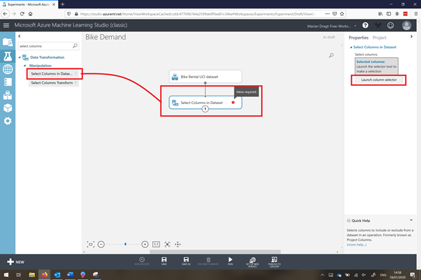
You can now select your desired variables by using the arrows. Make sure all variables except instant, casual and registered are in the ‘selected column’ (see picture below). Click on the ok sign right below when you are ready.

In order to see the results, you have to SAVE and RUN the model. You can find these options at the bottom menu of the page.

Step 5: Splitting the data

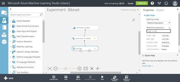
Now you are ready to split the dataset into a training dataset and a test dataset. You will train the model with 2011 data and test the model with 2012 data. Select the Split Data module and drag it on the canvas. Connect the output port of the Select Columns in Dataset module to the input port of the Split Data module. At the right, you can configure this module. In this case, we can use an expression to select 2011:

\"yr" == 0

Make sure you also set the correct Splitting mode. This will give you the 2011 data in the left (1) output port to train your model with, and the right (2) output port will contain the 2012 data to test your model with later. RUN the model and check your output data.

Step 6: Make sure you have all the required variables

Now we can remove the last variables that we don’t need anymore. We remove the year variable and the date variable. You can use the same procedure as before, by adding  the Select Columns in Dataset module and connecting the Split Data module to it.

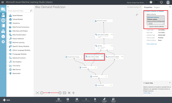
You can now select the variables that you need and leave those that you don’t.

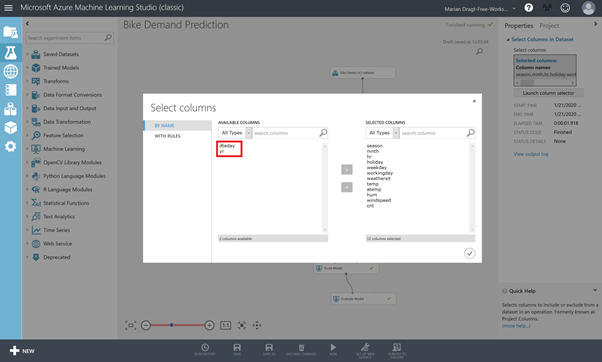
Make sure all variables except dteday and yr are in selected columns. Repeat this for both outputs of the Split Data module. You can copy-paste a module (right-click on a module) to lower your effort.

Step 7: Train the model

You are now ready to train the model. You need the Train Model module, an algorithm module, and the training dataset.

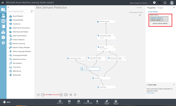
Drag the Train Model module on the canvas and connect the training dataset to it. Besides, drag the Boosted Decision Tree Regression algorithm on the canvas and connect it to the Train Model module. You can leave the pre-set hyperparameters as they are. In the Train Model module, make sure you select the dependent variable “cnt” to train the model on. Save and RUN your model.

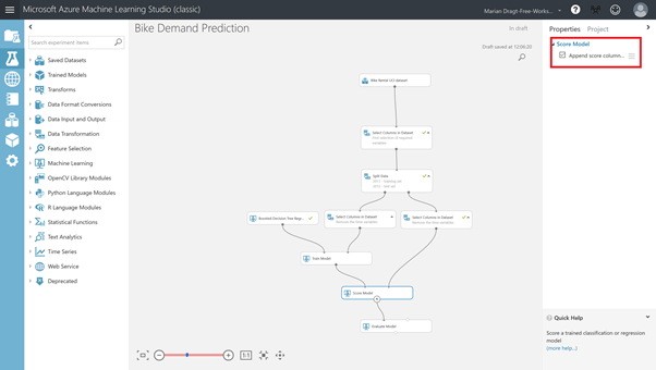
Step 8: Test the model

Now you have trained the model, and it’s time to test is. You can use your model to score the test dataset by dragging the Score Model module on the canvas and connecting it to the test dataset. By default, the results will be appended to the dataset. Save and run your model.

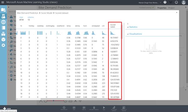
If you inspect the output of the Score Model module, by righ-clicking on the output port and selecting Visualize, you will see that there is an extra column in your dataset, named Scored Labels. This column contains the predicted number of rented bikes.

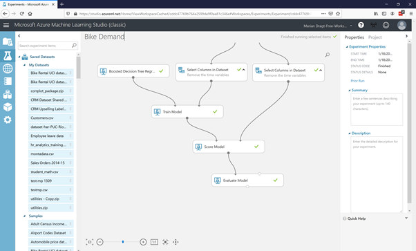
Step 9: Evaluate the model

As we also have the real number of rented bikes, we can make the evaluation. Luckily for us, there is a module that does the trick. Drag the Evaluate Model module on the canvas, connect it, and run your model. The Evaluate Model module has 2 input ports so you can compare models with each other. As we have only one model, make sure you connect it to the left input port.

After you have ran the model, you can inspect the results by right-clicking on the output port and choosing the Visualize options.

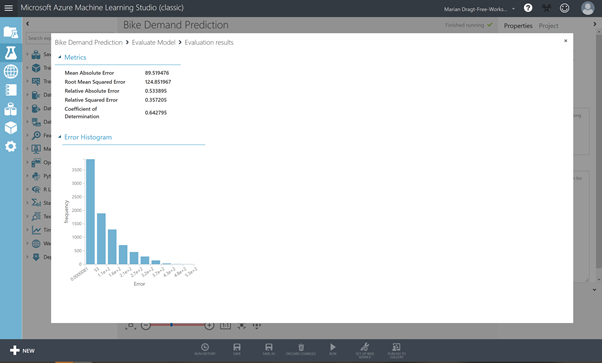
With this model, you can explain 64% of the variance in bike rental amount. Is that good enough? Well, that depends….

Step 10: Be sharp!

And here we come to the part where we look at the limitations and recommendations for future research.

First of all, we have skipped many steps which you would normally take when it comes to building a model. To start with, we would recommend you to understand the business question behind all this. Is predicting the number of rental bikes for a complete city really tell you something? Which business purpose are your serving? If we look at the original data source, you will find out that the original data also had the starting location and the ending location of the rental period. Now that starts to make sense: if we would be able to predict the amount of bikes for a specific location in the city, it could help the business to better stock their locations. Furthermore, we have skipped all the “normal” required steps for doing a regression: checking the distribution of the variables, the relations between them, outliers, etc. Now this was on purpose as this is a short workshop, but please make sure you do this right when you build a real model. Furthermore, based on the variables we have, we could create more features like i.e. amount of bikes rented the prior day, etc. This is up to your creativity.

Although there are quite some critical notes, we hope you have enjoyed this workshop and hopefully it inspired you to build your own models. If you want to take your models into production, then please use another environment: https://ml.azure.com/

Here you can find a similar interface, called Designer, but with this interface, you can also deploy and manage your models.