

Will somebody earn over 50k a year?
This workshop is about building a model to classify people using demographics to predict whether a person will have an annual income over 50K dollars or not.
The dataset used in this experiment is the US Adult Census Income Binary Classification dataset, which is a subset of the 1994 Census database, using working adults over the age of 16 with an adjusted income index of > 100.
This blog is inspired on the Sample 5: Binary Classification with Web Service: Adult Database from the Azure AI Gallery.
We will walk through the 10 steps to build the model, with an additional BONUS challenge to gain extra insights.
Step 1: Getting the data
Start with creating a new blank experiment. The data is directly available from the Azure Machine Learning sample datasets and is called the Adult Census Income Binary Classification dataset. You can drag this dataset on the canvas of your new experiment
We can get some quick data insights by using the standard visualization from the Azure Machine Learning studio:
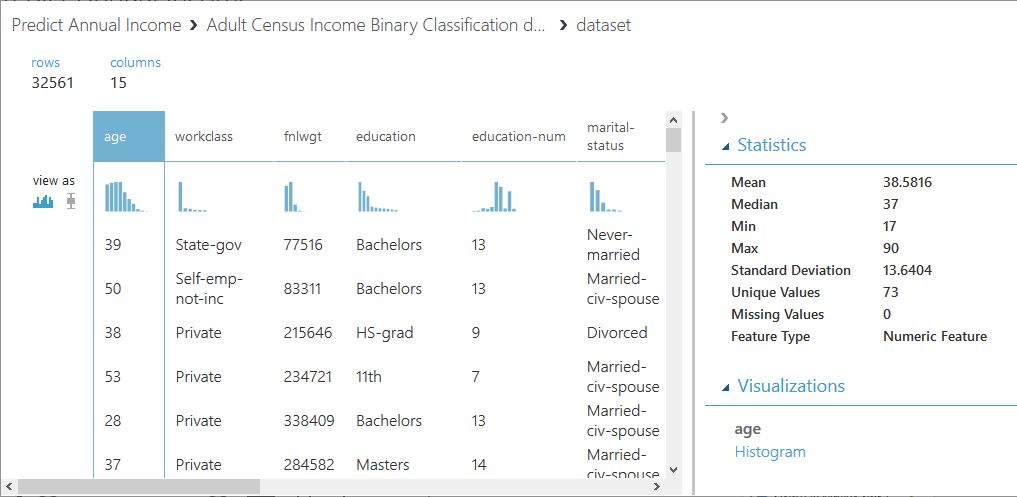
Step 2: Select required variables
First, we observe that “education” and “education-num” are equivalent. Based on the nature of the other variables, we decide to delete “education-num” and continue with “education”. Besides, as explained on the UCI Machine Learning Repository, we deleted the variable “fnlwgt”, which is a weighting variable that should not be used in classifiers.
Step 3: Clean missing data
For the categorical variables, we fill-out the missing values with the value “Other”. For the numerical variables, we replace the missing values with the median, as the mean would give a very distortionate view. Look i.e. at the variable “capital-gain”, where the mean is 1078 and the median 0. We end up with 1 dependent variable “income” and 12 predicting variables: “age”, “workclass”, “education”, “marital-status”, “occupation”, “relationship”, “race”, “sex”, “capital-gain”, “capital-loss”, “hours-per-week”, and “native-country”.
Step 4: Inspect the data
With the “Execute R Script” module we write a short script to show some basic graphs to better understand the available data. You can substitute the pregenerated code with the following code:
# Map 1-based optional input ports to variables
df <- maml.mapInputPort(1) # class: data.frame

# use ggplot 2 library for plotting
library(ggplot2)

  # make a plot for every column
cols <- 1:ncol(df)

 for(i in cols) {
   capture.output(
     ggplot(df, aes(df[,i], fill = df[,i] ) ) +
     geom_bar() +
     labs(x = colnames((df)[i])) +
     guides(fill=guide_legend(title=colnames((df)[i]))) +
     theme(axis.text.x = element_text(angle = 90, hjust = 1))
   ,file=NULL)
 }

# Select data.frame to be sent to the output Dataset port
maml.mapOutputPort("df");
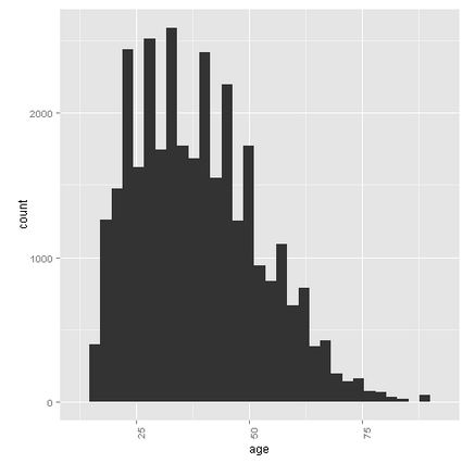
Age
The selection on the original database excludes people younger than 16. On average (both mean and median) one is 37/38 years old. However, there are quite some people over 75 that are stil working.
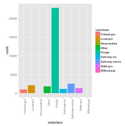
Workclass
Most of the people of this sample are from the private sector.
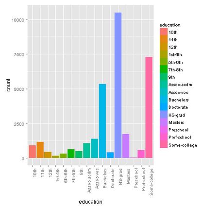
Education
Most of the people have a high-school degree or higher.
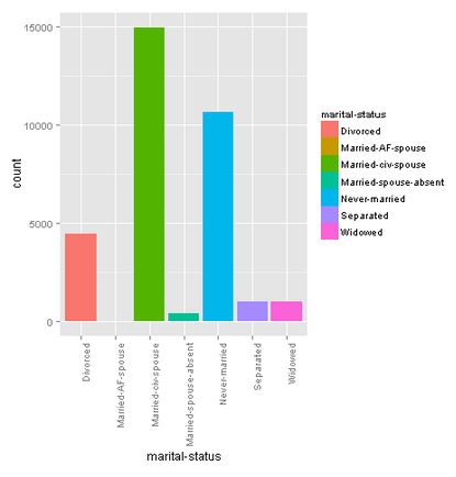
Marital-status
Many people are married (married-civ-spouse), followed by never-married people.
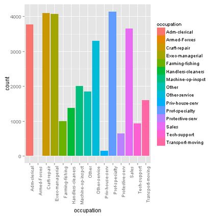
Occupation
There is quite a diversity among the occupation. We found 14 occupancies, and added an extra “other” option for those who left this field empty.
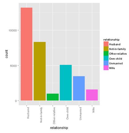
Relationship
Most of the people are found in a relationship as husband. This makes sense if we look at the gender distribution later on.
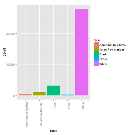
Race
The majority of this sample exists of white people.
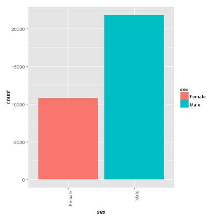
Sex
The male-female ratio is around 2:1. This also explains the high “husband” value for the “relationship” variable.
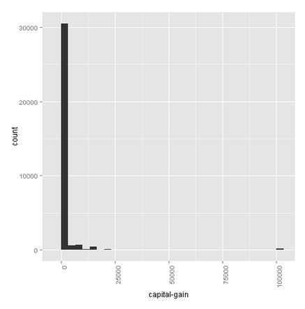
Capital-gain (currently not showing in Azure MLS)
There are very little people that have capital gains.
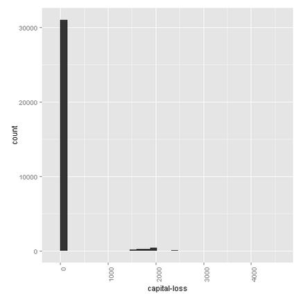
Capital-loss (Currently not showing in Azure MLS)
There are very little people that have capital losses.
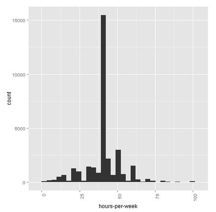
Hours-per-week
On average, one works 40 hours a week, although we see some very busy people with 100-hour weeks.
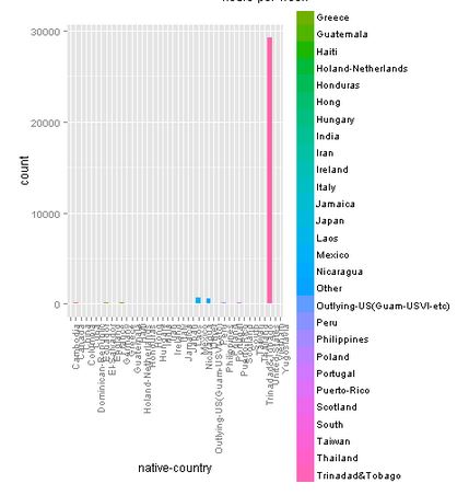
Native-country
This graph is not really clear in this environment. When running it in R (Studio), we can clearly see that most of the people are coming from the United States (the big pink bar).
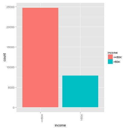
Income
76% of the sample earns less than 50K dollar a year, and 24% more. We will take this into account when splitting the data into a training and test set. We also set a seed to make this blog reproducible.
Step 5: Take care of the variable types
We make sure that we set the categorical variables from string to categorical. We will use this later on.
Step 6: Split the dataset into a training and a test set
We split the dataset into a training set with 70% of the data and a test set containing the other 30%, taking the income distribution into account by using a stratified split. We want to make this exercise repeatable and use “1234” as random seed.
Step 7: Train the basic model
For this experiment, we use the standard settings to train the model with a Two-Class Boosted Decision Tree algorithm. If you want to optimize theses settings in the future, you can tune them by using the Tune Model Hyperparameters module, but please take overfitting into account.
Step 8: Evaluate the Feature Importance
With the Feature Importance module, we can obtain the importance of the features. The scores are based on how much the performance of the model changes when the feature values are randomly shuffled. The scores that the module returns represent the change in the performance of a trained model, after permutation. Make it repeatable by setting the seed to “1”. We want to use Classification – Accuracy as metric for measuring performance.
With the help of an R script, we can display the scores of the features
# Map 1-based optional input ports to variables
df <- maml.mapInputPort(1) # class: data.frame

# Make sure the outcome score is numeric
df$Score <- as.numeric(df$Score)

# Plot the feature importancy scores
library(ggplot2)
p = ggplot(data=df, aes(x = Feature, y = Score))

# Reorder the features in the order of the score
df$Score2 <- reorder(df$Feature, df$Score)

capture.output( plot( p + geom_bar(aes(x=Score2), data=df, stat="identity") +
   coord_flip() +
   ggtitle("Importancy score per feature") ,
                 file = "NUL" ))

# Select data.frame to be sent to the output Dataset port
maml.mapOutputPort("df");
Question 1: What is the most important variable according to your model?
Question 2: Regarding the outcome of the feature importance scores, what do you think about the expression “Money makes money”?
Step 9: Score the test data
With the trained model, we score the test data.
Step 10: Evaluate the model
Finally, you can evaluate your trained model.
Question 3: What do you think about the results and why?
BONUS Challenge: Continuation of the Feature Importance
As we have seen in step 8, we have a better understanding of the importance of every feature. However, when it’s about categorical variables, it does not tell you if there is a specific value that drives this score.
Challenge: find a way to get more detailed information about the contribution of the categorical variables. Hint: you can convert categoricals…
I hope you enjoyed this experiment and I’m looking forward to hearing your opinion!
Related Research: Kohavi, R., Becker, B., (1996). UCI Machine Learning Repository http://archive.ics.uci.edu/ml. Irvine, CA: University of California, School of Information and Computer Science